# import os
# # Set working directory manually on Gadi to be able to load csv files
# user = os.getenv('USER')
# os.chdir('/scratch/cd82/'+user+'/notebooks/')🌳 Decision Tree Classification with Heart Disease Dataset
What is a Decision Tree?
A Decision Tree is a supervised machine learning model that splits the data into branches to make predictions. It works by asking a series of yes/no questions (based on features) to divide the data until a decision is made.
Key Concepts:
- Gini Impurity or Entropy is used to determine the best feature and threshold to split at each node.
- Decision Trees are interpretable, but they can overfit the training data.
Common Hyperparameters
max_depth: Limits how deep the tree can go (helps prevent overfitting).min_samples_split: Minimum number of samples required to split an internal node.min_samples_leaf: Minimum number of samples that a leaf node must have.
import pandas as pd
import numpy as np
import matplotlib.pyplot as plt
import seaborn as sns
from sklearn.tree import DecisionTreeClassifier, plot_tree
from sklearn.model_selection import train_test_split
from sklearn.metrics import classification_report, ConfusionMatrixDisplay, accuracy_score
import shap

# Load the dataset
df = pd.read_csv("heart.csv")
X = df.drop("target", axis=1)
y = df["target"]

# Train-test split
X_train, X_test, y_train, y_test = train_test_split(X, y, test_size=0.3, random_state=42)
🌲 Hyperparameter 1: max_depth
max_depth controls how deep the decision tree can grow. A shallow tree (e.g., max_depth=2) may underfit the data, while a very deep tree (e.g., None = no limit) may overfit the training set.
Below, we train several models with different max_depth values and observe the training and test accuracy.
depths = [2, 4, 6, 8, None]
train_scores, test_scores = [], []

for d in depths:
    clf = DecisionTreeClassifier(max_depth=d, random_state=42)
    clf.fit(X_train, y_train)
    train_scores.append(clf.score(X_train, y_train))
    test_scores.append(clf.score(X_test, y_test))

depth_labels = [str(d) if d is not None else "None" for d in depths]
plt.plot(depth_labels, train_scores, marker='o', label='Train Accuracy')
plt.plot(depth_labels, test_scores, marker='s', label='Test Accuracy')
plt.xlabel('max_depth')
plt.ylabel('Accuracy')
plt.title('Effect of max_depth on Accuracy')
plt.legend()
plt.grid(True)
plt.show()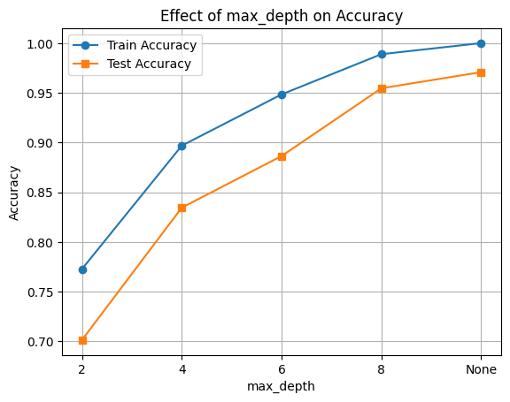
✂️ Hyperparameter 2: min_samples_split
This parameter defines the minimum number of samples required to split an internal node.
- Higher values prevent the tree from splitting too soon, which can reduce overfitting.
- Lower values allow the tree to grow deeper, which can increase accuracy but also risk overfitting.
Let’s observe how changing min_samples_split impacts model performance.
min_samples = [2, 5, 10, 20, 50]
train_scores, test_scores = [], []

for min_split in min_samples:
    clf = DecisionTreeClassifier(min_samples_split=min_split, random_state=42)
    clf.fit(X_train, y_train)
    train_scores.append(clf.score(X_train, y_train))
    test_scores.append(clf.score(X_test, y_test))

plt.plot(min_samples, train_scores, marker='o', label='Train Accuracy')
plt.plot(min_samples, test_scores, marker='s', label='Test Accuracy')
plt.xlabel('min_samples_split')
plt.ylabel('Accuracy')
plt.title('Effect of min_samples_split on Accuracy')
plt.legend()
plt.grid(True)
plt.show()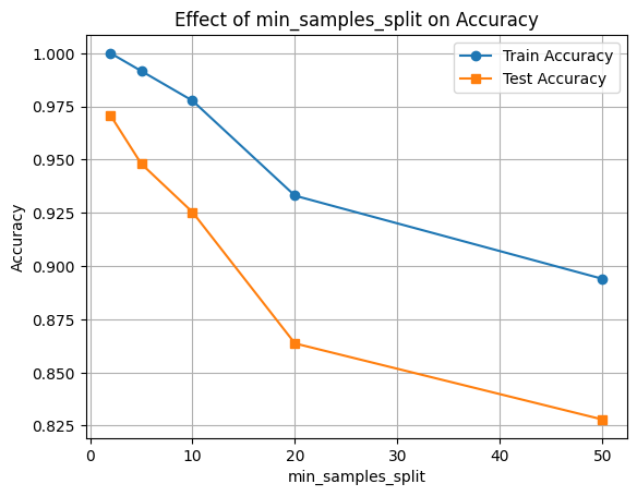
🍃 Hyperparameter 3: min_samples_leaf
This parameter controls the minimum number of samples required to be at a leaf node.
- It prevents the model from learning from very small subsets of data.
- Larger values make the model more conservative and help reduce overfitting.
We’ll now test how different values for min_samples_leaf affect the performance of our Decision Tree.
min_leaves = [1, 2, 5, 10, 20]
train_scores, test_scores = [], []

for min_leaf in min_leaves:
    clf = DecisionTreeClassifier(min_samples_leaf=min_leaf, random_state=42)
    clf.fit(X_train, y_train)
    train_scores.append(clf.score(X_train, y_train))
    test_scores.append(clf.score(X_test, y_test))

plt.plot(min_leaves, train_scores, marker='o', label='Train Accuracy')
plt.plot(min_leaves, test_scores, marker='s', label='Test Accuracy')
plt.xlabel('min_samples_leaf')
plt.ylabel('Accuracy')
plt.title('Effect of min_samples_leaf on Accuracy')
plt.legend()
plt.grid(True)
plt.show()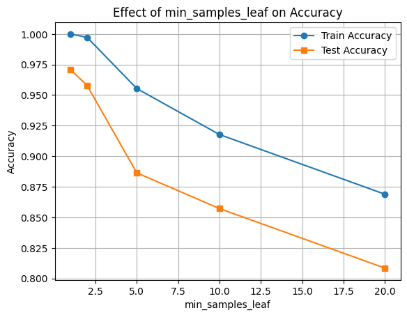
✅ Final Model with Selected Hyperparameters
We’ll now train a final Decision Tree model using the best combination of parameters observed in our experiments. Then we’ll use SHAP to interpret feature importance.
# Final model (tuned)
final_clf = DecisionTreeClassifier(max_depth=6, min_samples_split=10, min_samples_leaf=5, random_state=42)
final_clf.fit(X_train, y_train)

# Accuracy
train_acc = final_clf.score(X_train, y_train)
test_acc = final_clf.score(X_test, y_test)

print(f"Train Accuracy: {train_acc:.3f}")
print(f"Test Accuracy: {test_acc:.3f}")
Train Accuracy: 0.937
Test Accuracy: 0.873
y_pred = final_clf.predict(X_test)
print(classification_report(y_test, y_pred))
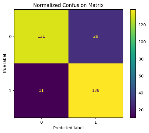
ConfusionMatrixDisplay.from_estimator(final_clf, X_test, y_test)
plt.title("Normalized Confusion Matrix")
plt.show() precision recall f1-score support
0 0.92 0.82 0.87 159
1 0.83 0.93 0.88 149
accuracy 0.87 308
macro avg 0.88 0.88 0.87 308
weighted avg 0.88 0.87 0.87 308
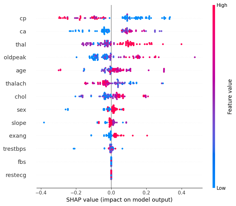
🧠 Feature Importance with SHAP
We’ll use SHAP (SHapley Additive exPlanations) to understand how different features contribute to the model’s predictions.
This helps us: - Identify the most influential features - Understand direction and magnitude of impact
📊 Interpreting the SHAP Summary Plot
The SHAP summary plot visualizes how each feature contributes to the model’s output across all samples. Here’s what each component means:
| Element | Description |
|---|---|
| Y-axis (Feature Names) | Features are sorted by overall importance (top = most important). |
| X-axis (SHAP value) | The impact of that feature on the model’s prediction. |
| Each Dot | A single row/sample in the dataset. |
| Color (Dot Hue) | The feature value for that sample — red = high, blue = low. |
| Direction of SHAP Value | Positive SHAP value pushes the prediction toward the positive class (e.g., “disease” class). |
| Negative SHAP value pushes it toward the negative class (e.g., “no disease”). |
🧠 Example Interpretation:
If the “Age” feature has mostly red dots (high values) with positive SHAP values, it means higher ages are pushing predictions toward the positive class.
import shap

explainer = shap.TreeExplainer(final_clf, X_train)

n_datapoints = 100
shap_values = explainer.shap_values(X_test[:n_datapoints])

class_index = 0
shap.summary_plot(shap_values[:, :, class_index], X_test[:n_datapoints])